CS231n Linear Classification 방식의 Image Classifier
Linear Classification 방식의 Image Classification을 만들어보았다.
# Image Classifier using Linear Classification method with Softmax and CIFAR 10 dataset

import numpy as np
import pickle
import matplotlib.pyplot as plt

# get batches from file
def get_batches(filename):
    with open(filename, 'rb') as file:
        data = pickle.load(file, encoding='bytes')

    return data

# activation function
def softmax(values):
    # prevent overflow
    values = values - np.max(values)
    return np.exp(values) / np.sum(np.exp(values))

# cross entropy loss? cost? function
def cross_entropy_loss(target_output, estimated_output):
    estimated_output = np.clip(estimated_output, 0.00001, 0.99999)
    return -np.mean(target_output * np.log(estimated_output) +
        (1 - target_output) * np.log(1 - estimated_output))

# train batches
def train():
    # make random wegith and bias
    W = np.random.rand(10, 3072)
    b = np.random.rand(10)

    # file_name_format
    file_prefix = 'cifar-10-batches-py/data_batch_{0}'

    for i in range(1, 6):
        # get batches
        batches = get_batches(file_prefix.format(i))

        for k in range(10000):
            # get batch
            x = batches[b'data'][k]
            # get output with Weight and bias using softmax activation function
            output = softmax(np.matmul(W, x) + b)

            # get answer
            answer = np.zeros(10)
            answer[batches[b'labels'][k]] = 1

            # get loss with answer and output using cross entropy loss function
            loss = cross_entropy_loss(answer, output)

            # update weight & bias

            # prevent "divided by zero exception"
            output_dc = np.clip(output, 0.00001, 0.99999)

            # dc/do : derivative of cross entropy loss function
            dc = (-answer / output_dc + (1 - answer) / (1 - output_dc)) / 10
            # do/dz : derivative of softmax function
            do = output_dc * (1 - output_dc)
            # dz/dw : derivative of z
            # z1 = w11 * x1 + w12 * x2 + ...
            # z1` = x1
            dz = np.copy(x)

            # do, dx, dz for updating weight
            do_w = np.repeat(do, 3072).reshape(10, 3072)
            dc_w = np.repeat(dc, 3072).reshape(10, 3072)
            dz_w = np.tile(dz, 10).reshape(10, 3072)

            # update weight (partial derivative of Cost function with respect to Weight)
            W -= dc_w * do_w * dz_w
            # update bias (partial derivative of Cost function with respect to Bias)
            b -= dc * do * 1

    # return Weight and bias
    return W, b

# predict
def predict(W, x, b):
    # get output using Neural Network
    output = softmax(np.matmul(W, x) + b)
    # argmax -> result
    return np.argmax(output)

if __name__ == "__main__":
    # get trained Weight and Bias
    W, b = train()

    # predict
    result = []

    # get test data
    batches = get_batches('cifar-10-batches-py/test_batch')
    for i in range(10000):
        # get single test image and label.
        x = batches[b'data'][i]
        y = batches[b'labels'][i]

        # get output from neural network
        y_ = predict(W, x, b)

        # add result to result list
        result.append(y_ == y)

    # get accuracy
    print("Accuracy : %f"%np.mean(np.array(result, dtype='float32')))

    # visualize weight and bias
    meta = get_batches('cifar-10-batches-py/batches.meta')

    for i in range(10):
        a = plt.subplot(2, 5, i + 1)
        a.set_title(meta[b'label_names'][i])
        I = np.copy(W[i]).reshape([-1, 1024]) + b[i]
        plt.imshow((I[0] * (2**16) + I[1] * (2**8) + I[2]).reshape(32, 32))

    plt.show()


# result
# Accuracy : 0.237800
소스코드는 위와 같고, 마지막 matplotlib으로 그려보면 다음과 같다.
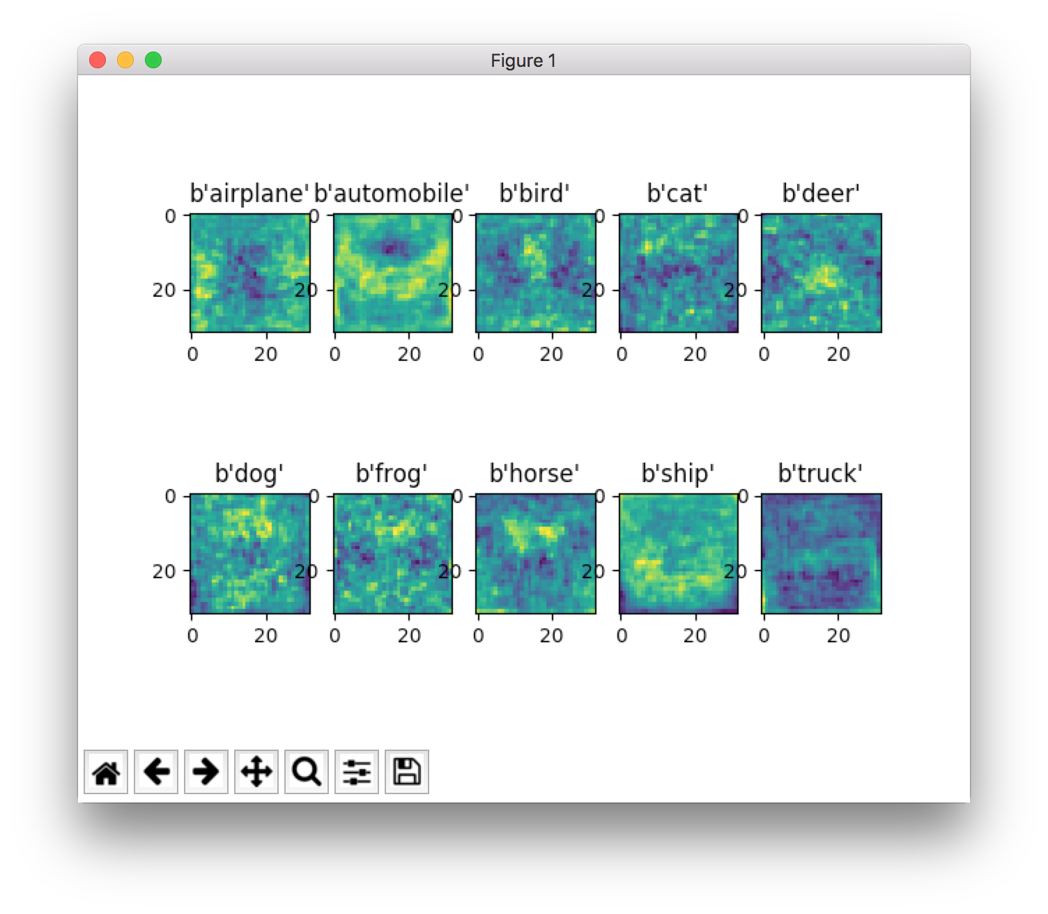
나름대로 horse은 대충 앞뒤로 서있는 것’처럼’ 보이고, automobile은 뭔가 앞면’처럼’ 보이고, ship은 바다위에 뭐가 있는 것’처럼’ 보인다고 생각 중이다.
neural network를 numpy로 처음 구현을 해보았는데, 생각보다 상당히 빠르게 학습을 하고 predict 과정도 생각보다 빨랐다. (레이어를 여러개를 쌓지 않아서 그런지는 모르겠지만)
앞의 KNN 방식과 비교를 하면, 강의 슬라이드에 적혀 있던 것처럼 학습이 좀 느리긴 느렸지만(학습이 30초정도 걸렸던 것 같다), 예측과정이 상당히 빨랐다. (KNN은 전체를 다 예측해볼 엄두도 내지 못했지만, 이번 방식으로는 다 학습시키고, 다 예측해보았으니)
근데 저 위의 소스코드가 저게 제대로 구현이 되었다고는 장담을 할 수가 없다. 단지 input, output layer만 있어서 정확도가 낮은건지, 아니면 뭔가 잘 못 구현해서 정확도가 낮은 것인지는 알 수가 없었다. 나중에 다른 것들도 구현을 해보면 뭐가 답이었는지는 나올 것 같다.
그래도 activation function, weight, bias, back propagation, loss function 등 여러가지 필수적인 부분들을 numpy만을 이용해서 직접 만들어보며 애매하게 넘어갔던 부분을 제대로 학습할 수 있었고(이론만은), 어떻게든 만들어 볼 수 있었다는 것에 의미가 있다고 생각한다.
SVM 부분은 제대로 이해를 못해서 아직 구현해보지 못했다.